Probability distributions with Python - Part 1
Introduction
L'objectif de cette quête est double : décrire certaines des distributions de probabilité les plus connues et présenter leur implémentation en Python. Dans la Partie 1, on va se concentrer sur les distributions de probabilité discrètes et explorer les fonctions de distribution Binomiale, de Bernoulli et de Poisson. Dans la Partie 2, on fera la même chose pour les distributions de probabilité continues et on explorera les distributions uniforme, normale, exponentielle et gamma.

🤓 À la fin de cette quête, tu sauras :
✅ Te familiariser avec 3 fonctions de distribution discrètes populaires : Bernoulli, Binomiale et Poisson ✅ Comprendre la définition formelle de ces fonctions de distribution ✅ Comprendre comment et quand utiliser ces fonctions ✅ Savoir utiliser le package (bibliothèque, ensemble de code réutilisable) SciPi de Python pour définir ces fonctions de distribution ✅ Savoir utiliser le package Seaborn de Python pour tracer ces fonctions de distribution
👀 Contenu de la quête :
- La fonction de distribution Binomiale
- La fonction de distribution de Bernoulli
- La fonction de distribution de Poisson
Pour un rappel sur les distributions de probabilité, les variables aléatoires discrètes et concrètes, les fonctions de densité de probabilité ou les fonctions de masse de probabilité, réfère-toi aux pré-requis ci-dessous.
Pré-requis
- Quête 1825 (hors archive)
- Quête 1826 (hors archive)
- Quête 1809 (hors archive)
👉Récupérer les bibliothèques Python nécessaires
Avant toute chose, chargeons les bibliothèques (libraries) nécessaires pour implémenter les distributions de probabilité avec Python
# for inline plots in jupyter, Colab or DeepNote
%matplotlib inline

# import matplotlib
import matplotlib.pyplot as plt

# for latex equations
from IPython.display import Math, Latex

# for displaying images
from IPython.core.display import Image

# import seaborn
import seaborn as sns

# settings for seaborn plotting style
sns.set(color_codes=True)

# settings for seaborn plot sizes
sns.set(rc={'figure.figsize':(5,5)})
👉La fonction de distribution Binomiale
Une distribution où seulement deux résultats sont possibles, comme succès ou échec, gain ou perte, victoire ou défaite, et où la probabilité de succès et d'échec est la même pour tous les essais, s'appelle une distribution Binomiale. Cependant, les résultats n'ont pas besoin d'être équiprobables, et chaque essai est indépendant des autres. Les paramètres d'une distribution binomiale sont $n$ et $p$, où $n$ est le nombre total d'essais, et $p$ la probabilité de succès à chaque essai.
Sa fonction de distribution de probabilité est donnée par : $$ f(k,n,p) = P(k;n,p) = P(X = k) = \binom{n}{k}p^k(1-p)^{n-k} $$
où :
$$ \binom{n}{k} = \frac{n!}{k!(n-k)!} $$
Implémentation en Python
Tu peux générer une variable aléatoire discrète suivant une loi binomiale avec la méthode binom.rvs() du module scipy.stats, qui prend $n$ (nombre d'essais) et $p$ (probabilité de succès) comme shape parameters (paramètres de forme, qui définissent l'allure de la distribution). Pour décaler la distribution, utilise le paramètre loc. size décide du nombre de fois où l'on répète les essais. Si tu veux garder la reproductibilité (pouvoir régénérer exactement les mêmes nombres), ajoute un argument random_state auquel tu assignes un nombre.
from scipy.stats import binom
data_binom = binom.rvs(n=10,p=0.8,size=10000)
Utilise distplot de seaborn pour visualiser sous forme d'histogramme la distribution que tu viens de créer
ax = sns.distplot(data_binom,
                  kde=False,
                  color='skyblue',
                  hist_kws={"linewidth": 15,'alpha':1})
ax.set(xlabel='Binomial Distribution', ylabel='Frequency')

# Formatting the text of the graph labels
[Text(0,0.5,u'Frequency'), Text(0.5,0,u'Binomial Distribution')]
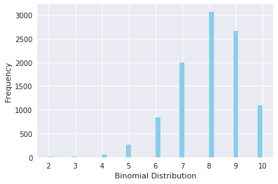
Remarque que, comme la probabilité de succès était supérieure à 0,5, la distribution est asymétrique (skewed) vers la droite. Il est aussi important de noter que la distribution de Poisson est un cas limite de la distribution binomiale sous les conditions suivantes :
- Le nombre d'essais est infiniment grand : n → ∞.
- La probabilité de succès à chaque essai est la même et infiniment petite : p → 0.
- np=λ est fini.
La distribution normale est une autre forme limite de la distribution binomiale sous les conditions suivantes :
- Le nombre d'essais est infiniment grand : n→∞
- p et q ne sont pas tous les deux infiniment petits
👉La fonction de distribution de Bernoulli
Une distribution de Bernoulli n'a que deux résultats possibles, à savoir $1$ (succès) et $0$ (échec), et un seul essai, par exemple un lancer de pièce. Donc la variable aléatoire $X$ qui suit une distribution de Bernoulli peut prendre la valeur $1$ avec la probabilité de succès $p$, et la valeur $0$ avec la probabilité d'échec $q$ ou $1−p$. Les probabilités de succès et d'échec n'ont pas besoin d'être équiprobables. La distribution de Bernoulli est un cas particulier de la distribution binomiale où un seul essai est réalisé (n=1). Sa fonction de masse de probabilité est donnée par :
$$ f(k;p) = p^k(1 - p)^{1-k}, for \space k \in {0, 1} $$
Tu peux générer une variable aléatoire discrète suivant une loi de Bernoulli avec la méthode bernoulli.rvs() du module scipy.stats, qui prend pp (probabilité de succès) comme shape parameter. Pour décaler la distribution, utilise le paramètre loc. size décide du nombre de fois où l'on répète les essais. Si tu veux garder la reproductibilité, ajoute un argument random_state auquel tu assignes un nombre.
from scipy.stats import bernoulli
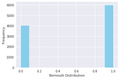
data_bern = bernoulli.rvs(size=10000,p=0.6)
Visualise la distribution avec seaborn.
ax= sns.distplot(data_bern,
                 kde=False,
                 color="skyblue",
                 hist_kws={"linewidth": 15,'alpha':1})
ax.set(xlabel='Bernoulli Distribution', ylabel='Frequency')
[Text(0,0.5,u'Frequency'), Text(0.5,0,u'Bernoulli Distribution')]
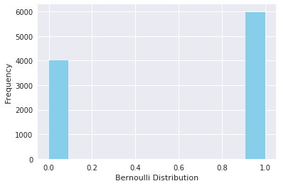
Le graphique montre que tu n'as que deux résultats possibles
👉La fonction de distribution de Poisson
Une variable aléatoire de Poisson est typiquement utilisée pour modéliser le nombre de fois qu'un événement s'est produit dans un intervalle de temps. Par exemple, le nombre de visites d'utilisateurs sur un site web dans un intervalle peut être vu comme un processus de Poisson. La distribution de Poisson est décrite en fonction du taux ($μ$) auquel les événements se produisent. Un événement peut se produire 0, 1, 2, … fois dans un intervalle. Le nombre moyen d'événements dans un intervalle est désigné par $λ$ (lambda). Lambda est le taux d'événements, aussi appelé rate parameter (paramètre de taux). La probabilité d'observer $k$ événements dans un intervalle est donnée par l'équation :
$$ P(k \space events \space in \space interval) = e^{-\lambda}\frac{\lambda^k}{k!} $$
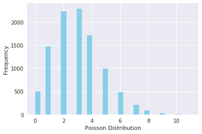
La figure suivante montre une distribution de Poisson typique :

Remarque que la distribution normale est un cas limite de la distribution de Poisson avec le paramètre λ → ∞. De plus, si les temps entre des événements aléatoires suivent une distribution exponentielle de taux λ, alors le nombre total d'événements sur une période de durée t suit la distribution de Poisson de paramètre λt.
Implémentation en Python
Tu peux générer une variable aléatoire discrète suivant une loi de Poisson avec la méthode poisson.rvs() du module scipy.stats, qui prend μμ comme shape parameter et qui n'est rien d'autre que le λλ de l'équation. Pour décaler la distribution, utilise le paramètre loc. size décide du nombre de variables aléatoires (random variates, les valeurs tirées au hasard) dans la distribution. Si tu veux garder la reproductibilité, ajoute un argument random_state auquel tu assignes un nombre.
from scipy.stats import poisson
data_poisson = poisson.rvs(mu=3, size=10000)
Ici aussi, tu peux visualiser la distribution sous forme d'histogramme avec les fonctions distplot de seaborn.
ax = sns.distplot(data_poisson,
                  bins=30,
                  kde=False,
                  color='skyblue',
                  hist_kws={"linewidth": 15,'alpha':1})
ax.set(xlabel='Poisson Distribution', ylabel='Frequency')
[Text(0,0.5,u'Frequency'), Text(0.5,0,u'Poisson Distribution')]
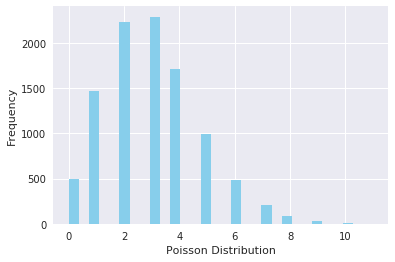
Explore la carte complète des fonctions de distribution discrètes et continues et la façon dont elles sont reliées entre elles
☝️ Résumé
Dans cette première partie de nos quêtes sur les Distributions de Probabilité avec Python, on a exploré la définition et l'implémentation en Python de 3 fonctions de distribution discrètes populaires : Bernoulli, Binomiale et Poisson.
Une distribution binomiale est une distribution où seulement deux résultats sont possibles (par exemple : succès ou échec, gain ou perte, victoire ou défaite) et où la probabilité de ces résultats est la même pour tous les essais. Une distribution de Bernoulli est une distribution avec seulement deux résultats possibles : 1 pour un succès et 0 pour un échec, et un seul essai. Une distribution de Poisson est utilisée quand la variable aléatoire se rapporte à un événement avec de nombreuses répétitions sur une période de temps.
Le module SciPi.stats contient les méthodes nécessaires pour définir ces distributions.
La méthode de scipi.stats pour la distribution binomiale est binom, pour Bernoulli c'est bernoulli et pour la distribution de Poisson, poisson.
La méthode displot de seaborn peut être utilisée pour tracer et visualiser ces distributions.
Tu peux explorer une carte détaillée de toutes les fonctions de distribution univariées et leurs relations ici.
💪 Challenge
Fais une copie de ce notebook Colab (carnet de code interactif) et réponds aux questions en mobilisant au mieux tes connaissances en distributions de probabilité et en Python.
Critères d'acceptation
- [ ] Utiliser SciPy pour répondre aux questions
- [ ] Fournir des explications de tes choix et de tes résultats
- [ ] Soumettre dans la quête un lien librement accessible vers ton notebook
Ressources supplémentaires
- Python for Data 22 : Distributions de probabilité
- Comment identifier la distribution de tes données
- Distributions de probabilité en Python avec SciPy et Seaborn
- Comment calculer et tracer une fonction de distribution cumulée avec Matplotlib en Python ?
- Tutoriel : Distributions de probabilité en Python
Introduction
The objective of this quest is two-folded: describe some of the most known probability distributions and present their implementation in Python. In Part 1, we will focus on discrete probability distribution and explore Binomial, Bernoulli, and Poisson distribution functions. In Part 2, we will do the same for the continuous probability distributions and explore uniform, normal, exponential, and gamma distributions.
🤓 By the end of this quest, you will:
✅ Get familiar with 3 popular discrete distribution functions: Bernoulli, Binomial, and Poisson ✅ Understand the formal definition of these distribution functions ✅ Understand how and when to use these functions ✅ Know how to use the Python's SciPi package to define these distribution functions ✅ Know how to use the Python's Seaborn package to plot these distribution functions
👀 Content of the quest:
- Binomial distribution function
- Bernoulli distribution function
- Poisson distribution function
For a refresher about probability distributions, discrete and concrete random variables, probability density functions or probability mass functions, please refer to the pre-requisites below.
Pre-requisites
- Quête 1825 (hors archive)
- Quête 1826 (hors archive)
- Quête 1809 (hors archive)
👉Getting the necessary Python libraries
First thing first, let's load the necessary libraries to implement probability distributions with Python
# for inline plots in jupyter, Colab or DeepNote
%matplotlib inline

# import matplotlib
import matplotlib.pyplot as plt

# for latex equations
from IPython.display import Math, Latex

# for displaying images
from IPython.core.display import Image

# import seaborn
import seaborn as sns

# settings for seaborn plotting style
sns.set(color_codes=True)

# settings for seaborn plot sizes
sns.set(rc={'figure.figsize':(5,5)})
👉Binomial distribution function
A distribution where only two outcomes are possible, such as success or failure, gain or loss, win or lose and where the probability of success and failure is the same for all the trials is called a Binomial Distribution. However, the outcomes need not be equally likely, and each trial is independent of each others. The parameters of a binomial distribution are $n$ and $p$ where $n$ is the total number of trials, and $p$ is the probability of success in each trial.
Its probability distribution function is given by : $$ f(k,n,p) = P(k;n,p) = P(X = k) = \binom{n}{k}p^k(1-p)^{n-k} $$
where:
$$ \binom{n}{k} = \frac{n!}{k!(n-k)!} $$
Python implementation
You can generate a binomial distributed discrete random variable using scipy.stats module's binom.rvs() method which takes $n$ (number of trials) and $p$ (probability of success) as shape parameters. To shift distribution use the loc parameter. size decides the number of times to repeat the trials. If you want to maintain reproducibility, include a random_state argument assigned to a number.
from scipy.stats import binom
data_binom = binom.rvs(n=10,p=0.8,size=10000)
Use seaborn's distplot to visualize as a histogram the distribution you just created
ax = sns.distplot(data_binom,
                  kde=False,
                  color='skyblue',
                  hist_kws={"linewidth": 15,'alpha':1})
ax.set(xlabel='Binomial Distribution', ylabel='Frequency')

# Formatting the text of the graph labels
[Text(0,0.5,u'Frequency'), Text(0.5,0,u'Binomial Distribution')]
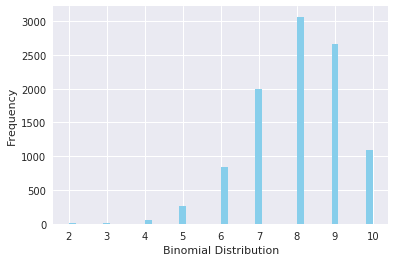
Note that since the probability of success was greater than 0.5 the distribution is skewed towards the right side. It is important to note as well that Poisson distribution is a limiting case of a binomial distribution under the following conditions:
- The number of trials is indefinitely large: n → ∞.
- The probability of success for each trial is the same and indefinitely small: p → 0.
- np=λ, is finite.
The normal distribution is another limiting form of binomial distribution under the following conditions:
- The number of trials is indefinitely large: n→∞
- Both p and q are not indefinitely small
👉Bernoulli distribution function
A Bernoulli distribution has only two possible outcomes, namely $1$ (success) and $0$ (failure), and a single trial, for example, a coin toss. So the random variable $X$ which has a Bernoulli distribution can take value $1$ with the probability of success, $p$, and the value $0$ with the probability of failure, $q$ or $1−p$. The probabilities of success and failure need not be equally likely. The Bernoulli distribution is a special case of the binomial distribution where a single trial is conducted (n=1). Its probability mass function is given by:
$$ f(k;p) = p^k(1 - p)^{1-k}, for \space k \in {0, 1} $$
You can generate a Bernoulli distributed discrete random variable using scipy.stats module's bernoulli.rvs() method which takes pp (probability of success) as a shape parameter. To shift distribution use the loc parameter. size decides the number of times to repeat the trials. If you want to maintain reproducibility, include a random_state argument assigned to a number.
from scipy.stats import bernoulli
data_bern = bernoulli.rvs(size=10000,p=0.6)
Visualize the distribution using seaborn.
ax= sns.distplot(data_bern,
                 kde=False,
                 color="skyblue",
                 hist_kws={"linewidth": 15,'alpha':1})
ax.set(xlabel='Bernoulli Distribution', ylabel='Frequency')
[Text(0,0.5,u'Frequency'), Text(0.5,0,u'Bernoulli Distribution')]
The graph shows that you have only two possible outcomes
👉Poisson distribution function
Poisson random variable is typically used to model the number of times an event happened in a time interval. For example, the number of users' visits on a website in an interval can be thought of as a Poisson process. Poisson distribution is described in terms of the rate ($μ$) at which the events happen. An event can occur 0, 1, 2, … times in an interval. The average number of events in an interval is designated by $λ$ (lambda). Lambda is the event rate, also called the rate parameter. The probability of observing $k$ events in an interval is given by the equation:
$$ P(k \space events \space in \space interval) = e^{-\lambda}\frac{\lambda^k}{k!} $$
The following figure shows a typical poisson distribution:
Note that the normal distribution is a limiting case of Poisson distribution with the parameter λ → ∞. Also, if the times between random events follow an exponential distribution with rate λ, then the total number of events in a time period of length t follows the Poisson distribution with parameter λt.
Python implementation
You can generate a poisson distributed discrete random variable using scipy.stats module's poisson.rvs() method which takes μμ as a shape parameter and is nothing but the λλ in the equation. To shift distribution use the loc parameter. size decides the number of random variates in the distribution. If you want to maintain reproducibility, include a random_state argument assigned to a number.
from scipy.stats import poisson
data_poisson = poisson.rvs(mu=3, size=10000)
Here as well you can visualize the distribution as an histogram using seaborn's distplot functions.
ax = sns.distplot(data_poisson,
                  bins=30,
                  kde=False,
                  color='skyblue',
                  hist_kws={"linewidth": 15,'alpha':1})
ax.set(xlabel='Poisson Distribution', ylabel='Frequency')
[Text(0,0.5,u'Frequency'), Text(0.5,0,u'Poisson Distribution')]
Explore the complete map of discrete and continuous distribution functions and how they are linked together
☝️ Summary
In this first part of our Probability Distributions with Python quests, we explored the definition and Python implementation of 3 popular discrete distribution functions: Bernoulli, Binomial and Poisson.
A binomial distribution is a distribution where only two outcomes are possible (e.g.: success or failure, gain or loss, win or lose) and where the probability of these outcomes is the same for all the trials. A Bernoulli distribution is a distribution with only two possible outcomes: 1 for success and 0 for failure, and a single trial. A Poisson distribution is used when the random variable refers to an event with numerous repetitions over a period of time.
The SciPi.stats module contains the necessary methods to define these distributions.
The method from scipi.stats for the binomial distribution is binom, for Bernouilli it is bernoulli and for Poisson distribution, poisson.
The method displot from seaborn can be used to plot and visualize these distributions.
You can explore an extensive map of all univariate distribution functions and their relationships here.
💪 Challenge
Make a copy of this Colab notebook and answer the questions using the best of your knowledge in probability distributions and Python.
Acceptance criteria
- [ ] Use SciPy to answer the questions
- [ ] Provide explainations of your choices and results
- [ ] Submit a freely accessible link to your notebook in the quest
More resources