Probability Distributions with Python - Part 2
Introduction
L'objectif de cette quête est double : décrire certaines des distributions de probabilité les plus connues et présenter leur implémentation (implementation : mise en œuvre concrète en code) et leur visualisation en Python. Dans la partie 1, nous avons exploré certaines des distributions de probabilité discrètes les plus populaires et leur implémentation, à savoir les distributions de Bernoulli, binomiale et de Poisson. Dans cette seconde partie, nous allons nous concentrer sur les distributions de probabilité continues et explorer la définition, l'implémentation et la visualisation des distributions uniforme, normale, exponentielle et gamma.
🤓 À la fin de cette quête, tu sauras :
✅ Te familiariser avec 4 fonctions de distribution continues populaires : uniforme, normale, exponentielle et gamma ✅ Comprendre la définition formelle de ces fonctions de distribution ✅ Comprendre comment et quand utiliser ces fonctions ✅ Savoir utiliser le package Python SciPi pour définir ces fonctions de distribution ✅ Savoir utiliser le package Python Seaborn pour tracer ces fonctions de distribution
👀 Contenu de la quête :
- Fonction de distribution uniforme
- Fonction de distribution normale
- Fonction de distribution exponentielle
- Fonction de distribution gamma
Pour une remise à niveau sur les distributions de probabilité, les variables aléatoires discrètes et concrètes, les fonctions de densité de probabilité ou les fonctions de masse de probabilité, réfère-toi aux pré-requis ci-dessous.
Pré-requis
- Quête 1825 (hors archive)
- Quête 1853
Récupérer les librairies Python nécessaires
Avant toute chose, chargeons les librairies nécessaires pour implémenter les distributions de probabilité avec Python
# for inline plots in jupyter, Colab or DeepNote
%matplotlib inline

# import matplotlib
import matplotlib.pyplot as plt

# for latex equations
from IPython.display import Math, Latex

# for displaying images
from IPython.core.display import Image

# import seaborn
import seaborn as sns

# settings for seaborn plotting style
sns.set(color_codes=True)

# settings for seaborn plot sizes
sns.set(rc={'figure.figsize':(5,5)})
👉Fonction de distribution uniforme
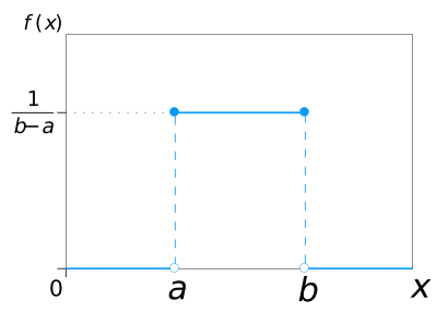
Dans une distribution uniforme, tout intervalle de nombres de même largeur a une probabilité égale d'être observé. Par conséquent, la courbe décrivant la distribution est un rectangle, avec une hauteur constante sur l'intervalle et une hauteur de 0 ailleurs. Comme l'aire sous la courbe doit être égale à 1, la longueur de l'intervalle détermine la hauteur de la courbe.
La figure suivante montre une distribution uniforme sur l'intervalle $(a,b)$. Remarque que, puisque l'aire doit valoir $1$, la hauteur est fixée à $1/(b−a)$.

Implémentation en Python
Tu peux visualiser les distributions uniformes en python à l'aide d'un générateur de nombres aléatoires agissant sur un intervalle de nombres (a,b). Pour cela, tu dois importer la fonction uniform depuis le module scipy.stats.
# import uniform distribution
from scipy.stats import uniform
La fonction uniform génère une variable continue uniforme sur l'intervalle spécifié via ses arguments loc et scale. Cette distribution est constante entre loc et loc + scale. L'argument size décrit le nombre de tirages aléatoires (random variates : réalisations aléatoires de la variable). Si tu veux garantir la reproductibilité, inclus un argument random_state auquel tu assignes un nombre.
# random numbers from a uniform distribution
n = 10000
start = 10
width = 20
data_uniform = uniform.rvs(size=n, loc = start, scale=width)
👉Fonction de distribution normale
La distribution normale, aussi appelée distribution gaussienne, est omniprésente en Data Science. Tu la rencontreras à de nombreux endroits, en particulier dans les sujets d'inférence statistique. C'est aussi l'une des hypothèses de beaucoup d'algorithmes de data science. Une distribution normale a une courbe de densité en forme de cloche décrite par sa moyenne $μ$ et son écart-type $σ$. La courbe de densité est symétrique, centrée autour de sa moyenne, avec son étalement déterminé par son écart-type, montrant que les données proches de la moyenne apparaissent plus fréquemment que les données éloignées de la moyenne. La fonction de distribution de probabilité d'une courbe de densité normale de moyenne $μ$ et d'écart-type $σ$ en un point donné $x$ est donnée par : $$ f(x|µ, σ^2) = \frac{1}{\sqrt{2 \pi σ^2}}e^{-\frac{(x-µ)^2}{2σ^2}} $$
Voici la figure décrivant à quoi ressemble la distribution :
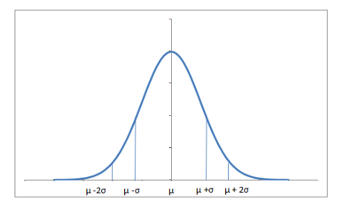 Près de 68% des données se situent à une distance d'un écart-type de la moyenne de part et d'autre, et 95% à moins de deux écarts-types.
Une distribution de moyenne 0 et d'écart-type 1 est appelée distribution normale centrée réduite.
Implémentation en Python
Tu peux générer une variable aléatoire distribuée normalement en utilisant la méthode norm.rvs() du module scipy.stats. L'argument loc correspond à la moyenne de la distribution. scale correspond à l'écart-type et size au nombre de tirages aléatoires. Si tu veux garantir la reproductibilité, inclus un argument random_state auquel tu assignes un nombre.
from scipy.stats import norm
# generate random numbers from N(0,1)
data_normal = norm.rvs(size=10000,loc=0,scale=1)
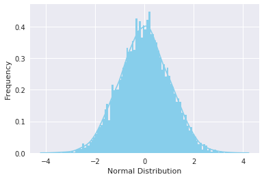
Tu peux visualiser la distribution comme d'habitude avec les fonctions distplot de seaborn. La signification des arguments reste la même que dans le cas précédent.
ax = sns.distplot(data_normal,
                  bins=100,
                  kde=True,
                  color='skyblue',
                  hist_kws={"linewidth": 15,'alpha':1})
ax.set(xlabel='Normal Distribution', ylabel='Frequency')
[Text(0,0.5,u'Frequency'), Text(0.5,0,u'Normal Distribution')]
👉Fonction de distribution exponentielle
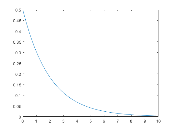
La distribution exponentielle décrit le temps entre des événements dans un processus ponctuel de Poisson, c'est-à-dire un processus dans lequel les événements se produisent de manière continue et indépendante à un taux moyen constant. Elle a un paramètre $λ$ appelé paramètre de taux (rate parameter), et son équation est décrite ainsi :
$$ f(x;λ) = {{^{λe^{-λx} \space \space x \ge 0}_{0 \space \space \space \space \space \space \space \space \space \space x < 0 }} $$
Une distribution exponentielle décroissante ressemble à :
Implémentation en Python
Tu peux générer une variable aléatoire distribuée exponentiellement en utilisant la méthode expon.rvs() du module scipy.stats. Cette méthode prend le paramètre de forme scale comme argument, lequel représente le $\lambda$ de l'équation. Pour décaler la distribution, utilise l'argument loc, size décide du nombre de tirages aléatoires dans la distribution. Si tu veux garantir la reproductibilité, inclus un argument random_state.
from scipy.stats import expon
data_expon = expon.rvs(scale=1,loc=0,size=1000)
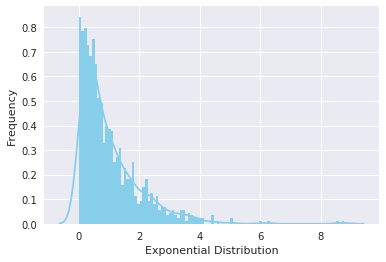
Encore une fois, visualiser la distribution avec seaborn donne la courbe montrée ci-dessous :
ax = sns.distplot(data_expon,
                  kde=True,
                  bins=100,
                  color='skyblue',
                  hist_kws={"linewidth": 15,'alpha':1})
ax.set(xlabel='Exponential Distribution', ylabel='Frequency')
[Text(0,0.5,u'Frequency'), Text(0.5,0,u'Exponential Distribution')]
👉Fonction de distribution gamma
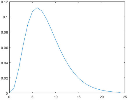
La distribution gamma est une distribution de probabilité continue à deux paramètres. Elle est rarement utilisée sous sa forme brute mais elle est très populaire comme base d'autres distributions largement utilisées. En fait, les distributions exponentielle, du chi-deux (chi-squared) ou d'Erlang sont des cas particuliers de la distribution gamma. Les paramètres de la distribution gamma incluent un paramètre de forme $α=k$ et un paramètre d'échelle inverse $β=1/θ$, appelé paramètre de taux. Le symbole $Γ(n)$ est la fonction gamma et est définie par $(n−1)!$. Formellement : $$ f(x; α,β) = \frac{β^{α}x^{α-1}e^{-βx}}{Γ(α)} \space \space for \space x>0 \space and \space α, β>0 $$
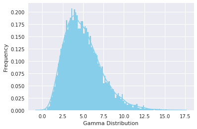
Une distribution gamma typique ressemble à :
Implémentation en Python
Tu peux générer une variable aléatoire distribuée selon une loi gamma en utilisant la méthode gamma.rvs() du module scipy.stats. Elle prend en argument le paramètre de forme $a$. Quand $a$ est un entier, gamma se réduit à la distribution d'Erlang, et quand $a=1$, elle se réduit à la distribution exponentielle. Pour décaler la distribution, utilise l'argument loc, pour la mettre à l'échelle, utilise l'argument scale. L'argument size décide du nombre de tirages aléatoires dans la distribution. Si tu veux garantir la reproductibilité, inclus un argument random_state.
from scipy.stats import gamma
data_gamma = gamma.rvs(a=5, size=10000)
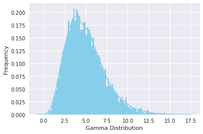
Utilise la fonction distplot de seaborn pour visualiser la distribution.
ax = sns.distplot(data_gamma,
                  kde=True,
                  bins=100,
                  color='skyblue',
                  hist_kws={"linewidth": 15,'alpha':1})
ax.set(xlabel='Gamma Distribution', ylabel='Frequency')
[Text(0,0.5,u'Frequency'), Text(0.5,0,u'Gamma Distribution')]
Explore la carte complète des fonctions de distribution discrètes et continues et la façon dont elles sont liées entre elles
☝️ Résumé
Dans cette seconde partie de nos quêtes sur les distributions de probabilité avec Python, nous avons exploré la définition et l'implémentation en Python de 4 fonctions de distribution continues populaires : uniforme, normale, exponentielle et gamma.
- Dans une distribution uniforme, tout intervalle de nombres de même largeur a une probabilité égale d'être observé. Sa courbe de densité est un rectangle avec une hauteur constante sur l'intervalle et une hauteur de 0 ailleurs.
- La distribution normale, aussi connue sous le nom de distribution gaussienne, définit une courbe de densité symétrique, centrée autour de sa moyenne, avec son étalement déterminé par son écart-type : les données proches de la moyenne sont plus fréquentes que les données plus éloignées de la moyenne.
- La distribution exponentielle décrit le temps entre des événements dans un processus où les événements se produisent de manière continue et indépendante à un taux moyen constant.
- La distribution gamma est une distribution de probabilité continue à deux paramètres qui sert de formalisation générale des distributions exponentielle, du chi-deux ou d'Erlang.
Le module SciPy.stats contient les méthodes nécessaires pour définir ces distributions.
La méthode de scipy.stats pour la distribution uniforme est uniform, pour la distribution normale c'est norm, pour l'exponentielle c'est expon, et pour la distribution gamma, gamma.
La méthode displot de seaborn peut être utilisée pour tracer et visualiser ces distributions.
Tu peux explorer une carte étendue de toutes les fonctions de distribution univariées et leurs relations ici.
💪 Défi
Fais une copie de ce notebook Colab et réponds aux questions en utilisant au mieux tes connaissances en distributions de probabilité et en Python.
Critères d'acceptation
- [ ] Utiliser SciPy pour répondre aux questions
- [ ] Fournir des explications de tes choix et de tes résultats
- [ ] Soumettre un lien librement accessible vers ton notebook à la fin de la quête
Introduction
The objective of this quest is two-folded: describe some of the most known probability distributions and present their implementation and visualization in Python. In Part 1, we explored some of the most popular discrete probability distributions and their implementation, namely, Bernoulli, Binomial, and Poisson distributions. In this second part, we will focus on the continuous probability distributions and explore the definition, implementation and visualization of the uniform, normal, exponential, and gamma distributions.
🤓 By the end of this quest, you will:
✅ Get familiar with 4 popular continuous distribution functions: uniform, normal, exponential and gamma ✅ Understand the formal definition of these distribution functions ✅ Understand how and when to use these functions ✅ Know how to use the Python's SciPi package to define these distribution functions ✅ Know how to use the Python's Seaborn package to plot these distribution functions
👀 Content of the quest:
- Uniform distribution function
- Normal distribution function
- Exponential distribution function
- Gamma distribution function
For a refresher about probability distributions, discrete and concrete random variables, probability density functions or probability mass functions, please refer to the pre-requisites below.
Pre-requisites
- Quête 1825 (hors archive)
- Quête 1853
Getting the necessary Python libraries
First thing first, let's load the necessary libraries to implement probability distributions with Python
# for inline plots in jupyter, Colab or DeepNote
%matplotlib inline

# import matplotlib
import matplotlib.pyplot as plt

# for latex equations
from IPython.display import Math, Latex

# for displaying images
from IPython.core.display import Image

# import seaborn
import seaborn as sns

# settings for seaborn plotting style
sns.set(color_codes=True)

# settings for seaborn plot sizes
sns.set(rc={'figure.figsize':(5,5)})
👉Uniform Distribution Function
In a uniform distribution, any interval of numbers of equal width has an equal probability of being observed. As a consequence, the curve describing the distribution is a rectangle, with constant height across the interval and 0 height elsewhere. Since the area under the curve must be equal to 1, the length of the interval determines the height of the curve.
The following figure shows a uniform distribution in the interval $(a,b)$. Notice since the area needs to be $1$. The height is set to $1/(b−a)$.
Python implementation
You can visualize uniform distributions in python with the help of a random number generator acting over an interval of numbers (a,b). To do that, you need to import the uniform function from scipy.stats module.
# import uniform distribution
from scipy.stats import uniform
The uniform function generates a uniform continuous variable between the specified interval via its loc and scale arguments. This distribution is constant between loc and loc + scale. The size arguments describe the number of random variates. If you want to maintain reproducibility, include a random_state argument assigned to a number.
# random numbers from a uniform distribution
n = 10000
start = 10
width = 20
data_uniform = uniform.rvs(size=n, loc = start, scale=width)
👉Normal distribution function
Normal Distribution, also known as Gaussian distribution, is ubiquitous in Data Science. You will encounter it at many places especially in topics of statistical inference. It is one of the assumptions of many data science algorithms too. A normal distribution has a bell-shaped density curve described by its mean $μ$ and standard deviation $σ$. The density curve is symmetrical, centered about its mean, with its spread determined by its standard deviation showing that data near the mean are more frequent in occurrence than data far from the mean. The probability distribution function of a normal density curve with mean $μ$ and standard deviation $σ$ at a given point $x$ is given by: $$ f(x|µ, σ^2) = \frac{1}{\sqrt{2 \pi σ^2}}e^{-\frac{(x-µ)^2}{2σ^2}} $$
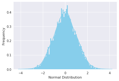
Below is the figure describing what the distribution looks like:
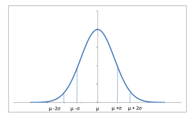 Almost 68% of the data falls within a distance of one standard deviation from the mean on either side and 95% within two standard deviations.
A distribution with mean 0 and standard deviation 1 is called a standard normal distribution.
Python implementation
You can generate a normally distributed random variable using scipy.stats module's norm.rvs() method. The loc argument corresponds to the mean of the distribution. scale corresponds to standard deviation and size to the number of random variates. If you want to maintain reproducibility, include a random_state argument assigned to a number.
from scipy.stats import norm
# generate random numbers from N(0,1)
data_normal = norm.rvs(size=10000,loc=0,scale=1)
You can visualize the distribution as usual with the seaborn's distplot functions. The meaning of the arguments remains the same as in the last case.
ax = sns.distplot(data_normal,
                  bins=100,
                  kde=True,
                  color='skyblue',
                  hist_kws={"linewidth": 15,'alpha':1})
ax.set(xlabel='Normal Distribution', ylabel='Frequency')
[Text(0,0.5,u'Frequency'), Text(0.5,0,u'Normal Distribution')]
👉Exponential distribution function
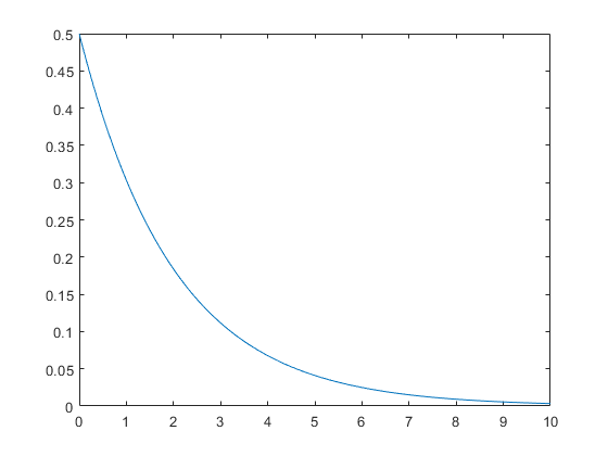
The exponential distribution describes the time between events in a Poisson point process, i.e., a process in which events occur continuously and independently at a constant average rate. It has a parameter $λ$ called rate parameter, and its equation is described as:
$$ f(x;λ) = {{^{λe^{-λx} \space \space x \ge 0}_{0 \space \space \space \space \space \space \space \space \space \space x < 0 }} $$
A decreasing exponential distribution looks like:
Python implementation
You can generate an exponentially distributed random variable using the method expon.rvs() from the module scipy.stats. This method takes the shape parameter scale as its argument which represents the $\lambda$ of the equation. To shift distribution, use the loc argument, size decides the number of random variates in the distribution. If you want to maintain reproducibility, include a random_state argument.
from scipy.stats import expon
data_expon = expon.rvs(scale=1,loc=0,size=1000)
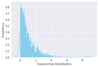
Again visualizing the distribution with seaborn yields the curve shown below:
ax = sns.distplot(data_expon,
                  kde=True,
                  bins=100,
                  color='skyblue',
                  hist_kws={"linewidth": 15,'alpha':1})
ax.set(xlabel='Exponential Distribution', ylabel='Frequency')
[Text(0,0.5,u'Frequency'), Text(0.5,0,u'Exponential Distribution')]
👉Gamma distribution function
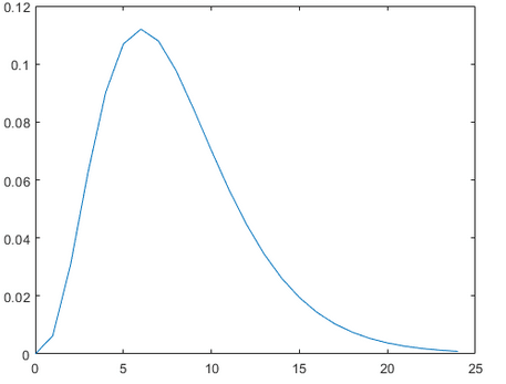
The gamma distribution is a two-parameter continuous probability distribution. It is rarely used in its raw form but it is very popular as the basis of other widely used distributions. In fact, exponential, chi-squared, or erlang distributions are special cases of the gamma distribution. The gamma distribution parameters include a shape parameter $α=k$ and an inverse scale parameter $β=1/θ$, called a rate parameter. The symbol $Γ(n)$ is the gamma function and is defined as $(n−1)!$. Formally: $$ f(x; α,β) = \frac{β^{α}x^{α-1}e^{-βx}}{Γ(α)} \space \space for \space x>0 \space and \space α, β>0 $$
A typical gamma distribution looks like:
Python implementation
You can generate a gamma distributed random variable using the method gamma.rvs() of the module scipy.stats. It takes in argument the shape parameter $a$. When $a$ is an integer, gamma reduces to the Erlang distribution, and when $a=1$, it reduces to the exponential distribution. To shift distribution, use the loc argument, to scale, use the scale argument. The argument size decides the number of random variates in the distribution. If you want to maintain reproducibility, include a random_state argument.
from scipy.stats import gamma
data_gamma = gamma.rvs(a=5, size=10000)
Use the distplot function from seaborn to visualize the distribution.
ax = sns.distplot(data_gamma,
                  kde=True,
                  bins=100,
                  color='skyblue',
                  hist_kws={"linewidth": 15,'alpha':1})
ax.set(xlabel='Gamma Distribution', ylabel='Frequency')
[Text(0,0.5,u'Frequency'), Text(0.5,0,u'Gamma Distribution')]
Explore the complete map of discrete and continuous distribution functions and how they are linked together
☝️ Summary
In this second part of our Probability Distributions with Python quests, we explored the definition and Python implementation of 4 popular continuous distribution functions: uniform, normal, exponential and gamma.
- In a uniform distribution, any interval of numbers of equal width has an equal probability of being observed. Its density curve is a rectangle with constant height across the interval and 0 height elsewhere.
- The normal distribution, also known as gaussian distribution defines a symmetrical density curve, centered around its mean, with its spread determined by its standard deviation: data near the mean are more frequent than data further away from the mean.
- The exponential distribution describes the time between events in a process where events occur continuously and independently at a constant average rate.
- The gamma distribution is a two-parameter continuous probability distribution that serves as a general formalization of exponential, chi-squared, or erlang distributions.
The SciPy.stats module contains the necessary methods to define these distributions.
The method from scipy.stats for the uniform distribution is uniform, for the normal distribution, it is norm, for the exponential one it is expon, and for the gamma distribution, gamma.
The method displot from seaborn can be used to plot and visualize these distributions.
You can explore an extensive map of all univariate distribution functions and their relationships here.
💪 Challenge
Make a copy of this Colab notebook and answer the questions using the best of your knowledge in probability distributions and Python.
Acceptance criteria
- [ ] Use SciPy to answer the questions
- [ ] Provide explainations of your choices and results
- [ ] Submit a freely accessible link to your notebook in the quest