Exploring graphs with Python
Introduction
« Une image vaut mille mots » est l'une des phrases les plus utilisées. Mais un graphique en dit bien plus encore. Une représentation visuelle des données, sous forme de graphiques, nous aide à tirer des enseignements concrets et à prendre de meilleures décisions fondées sur les données.

🤓 À la fin de cette quête, tu sauras :
✅ Comprendre quelques applications courantes des graphes ✅ Savoir créer et gérer des graphes avec Python ✅ Comprendre comment utiliser GraphViz pour visualiser des graphes
👀 Contenu de la quête :
- Rappel sur la définition d'un graphe
- Applications courantes des graphes
- Création de graphes avec Python
- Visualisation de graphes avec Python
- Exploration d'un jeu de données avec des graphes
- Exploration avec NetworkX
- Identification des plus courts chemins
👉 Rappel sur la définition d'un graphe
Définition de base d'un graphe
Les graphes sont des structures mathématiques utilisées pour étudier les relations deux à deux entre des objets et des entités. C'est une branche des mathématiques discrètes qui a trouvé de nombreuses applications en informatique, chimie, linguistique, recherche opérationnelle, sociologie, etc. Il en va de même en Data Science et en analyse de données, où les graphes servent à modéliser diverses structures et problèmes.
Regardons un graphe simple pour revoir le concept. Observe l'image ci-dessous. Imagine que ce graphe représente les lieux d'une ville que les gens visitent généralement, ainsi que le chemin suivi par un visiteur de cette ville.
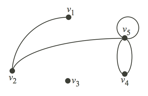
Considérons V comme les lieux et E comme le chemin pour aller d'un lieu à un autre.
V = {v1, v2, v3, v4, v5}

E = {(v1,v2), (v2,v5), (v5, v5), (v4,v5), (v4,v4)}
Ici, l'arête (u,v) est la même que l'arête (v,u) : ce sont des paires non ordonnées.
Formellement, un graphe (graph : structure reliant des objets par des liens) est un couple d'ensembles tel que G = (V,E). V est l'ensemble des sommets (vertices : les points du graphe) et E, un ensemble d'arêtes (edges : les liens entre les sommets). E est constitué de paires d'éléments de V (paire non ordonnée). Dans certains cas, il est important de considérer les arêtes comme des paires ordonnées. On appelle alors généralement ces arêtes des arcs pour marquer la notion de direction, et ces graphes sont appelés des digraphes (digraph : graphe orienté). Formellement, un digraphe est un couple d'ensembles tel que D = (V,A). V est l'ensemble des sommets et A, l'ensemble des arcs. A est constitué de paires d'éléments de V (paire ordonnée).
Dans un digraphe, (u,v) est différent de (v,u).
R et Python proposent des paquets pour analyser des données à l'aide des concepts de la théorie des graphes. Dans cette quête, nous utiliserons le paquet Python NetworkX.
Composants d'un graphe
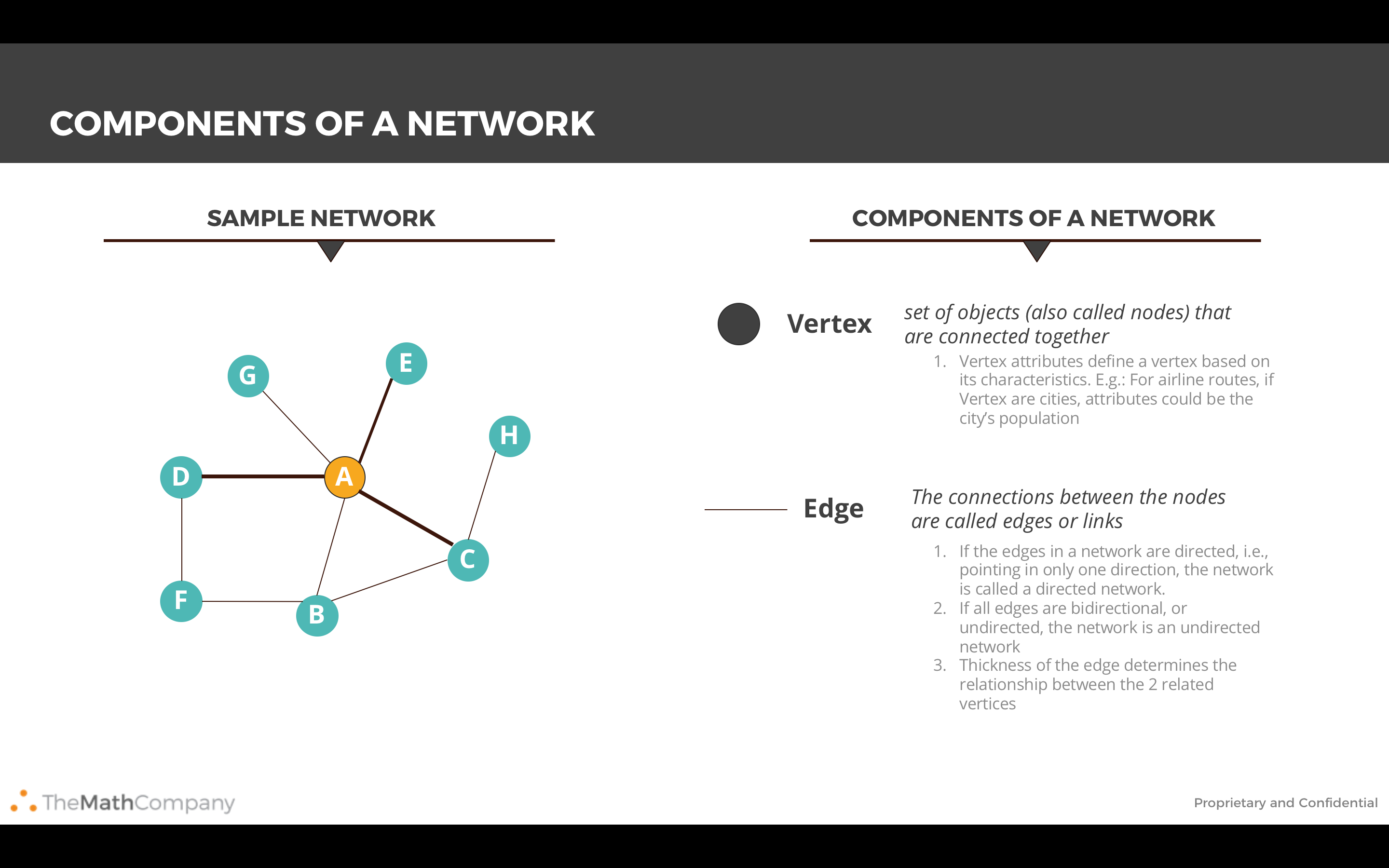
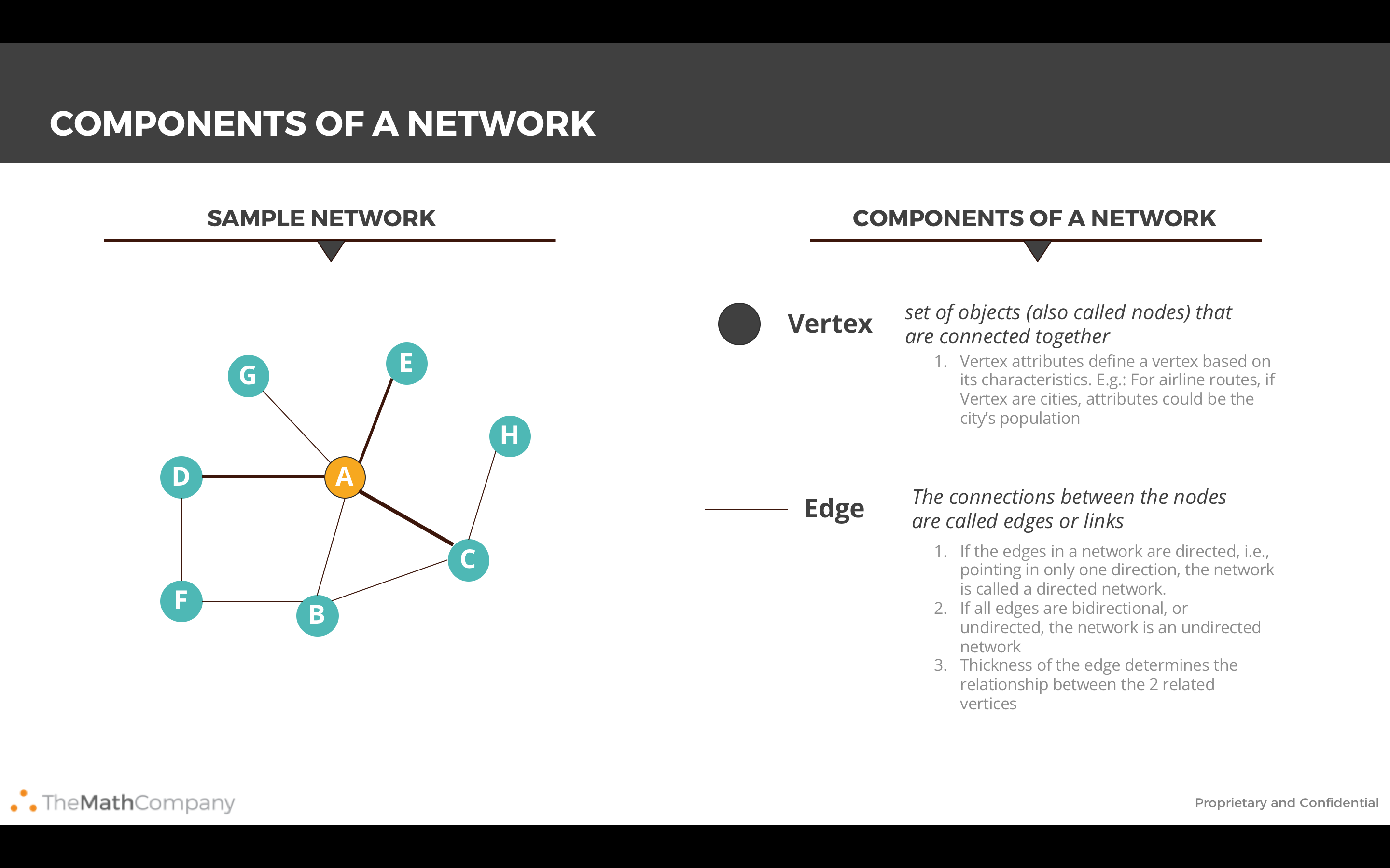
Python tient à notre disposition des rappels rapides sur les graphes, auxquels on peut accéder via l'affichage du paquet natif. Voici par exemple un résumé de la composition d'un graphe. Note que graphe et réseau (network) sont utilisés de manière interchangeable ici. Il n'y a pas de différence entre les deux, si ce n'est la nécessité de considérer le réseau comme l'implémentation (programmatique) d'un graphe (mathématique).
from IPython.display import Image
Image('images/network.PNG')
👉 Applications courantes des graphes
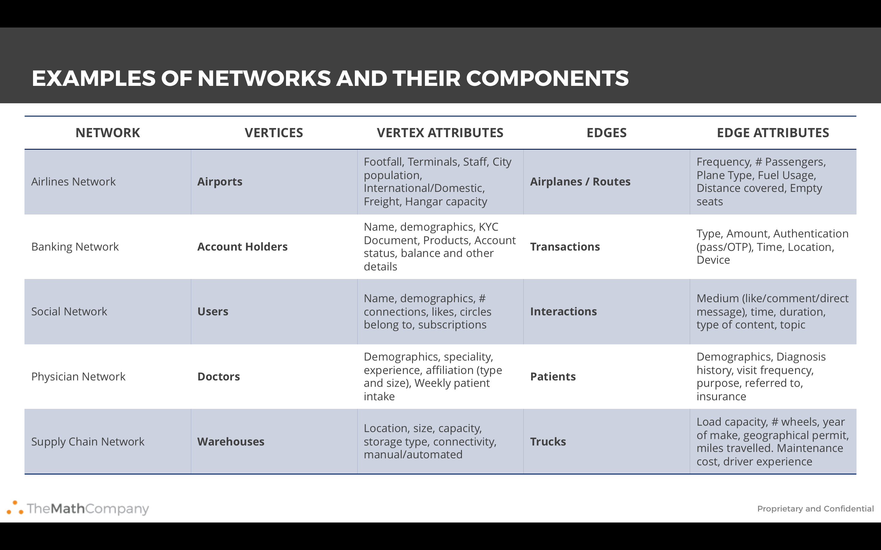
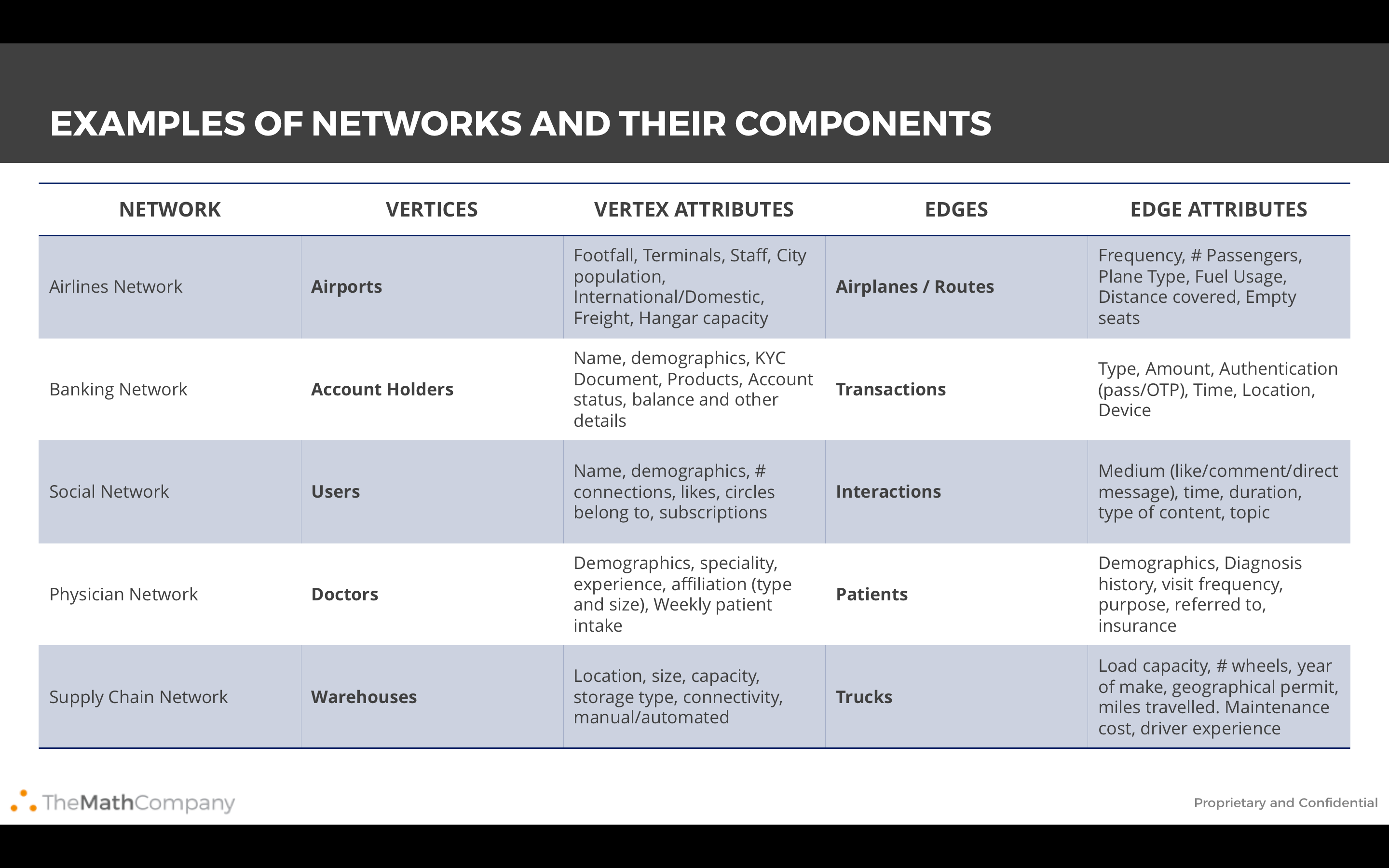
Les graphes sont largement utilisés pour modéliser, analyser et résoudre des problèmes de la vie réelle. Ici, tu trouveras quelques exemples d'applications notables de la théorie des graphes à des problèmes courants.
Image('images/usecase.PNG')
Quelques applications supplémentaires qui méritent d'être citées :
- Marketing analytique : les graphes peuvent servir à repérer les personnes les plus influentes d'un réseau social. Les annonceurs et les spécialistes du marketing peuvent ainsi estimer la meilleure performance pour leurs campagnes en faisant passer leur message par les personnes les plus influentes.
- Transactions bancaires : les graphes peuvent servir à détecter des schémas inhabituels, ce qui aide à limiter les transactions frauduleuses. Dans certains cas, le financement d'activités terroristes a été détecté en analysant les flux d'argent à travers des réseaux bancaires interconnectés.
- Chaîne d'approvisionnement : les graphes aident à identifier les itinéraires optimaux pour les camions de livraison ainsi que les emplacements optimaux pour les entrepôts et les centres de livraison.
- Télécom : les entreprises de télécommunications utilisent généralement des graphes (diagrammes de Voronoï) pour optimiser la couverture des antennes-relais sur une surface géographique donnée.
👉 Création de graphes avec Python
Nous allons utiliser le paquet networkx en Python. Ce paquet doit être installé avant utilisation.
Regardons quelques opérations courantes que nous pouvons réaliser avec le paquet NetworkX.
Création d'un graphe
import networkx as nx

# Create a Graph
G = nx.Graph() # This create a Graph object G but it is empty for now

# Add a node
G.add_node(1)

# Add a list of nodes by passing a list argument
G.add_nodes_from([2,3])

# Add edges between nodes
G.add_edge(1,2)

e = (2,3)
G.add_edge(*e) # the symbol * is used to unpack the tuple

# We can add edges using lists as well
G.add_edges_from([(1,2), (1,3)])
Voici quelques fonctions NetworkX supplémentaires qui peuvent se révéler pratiques pour créer, traiter et gérer des graphes :
| Fonction | Description |
|---|---|
| subgraph(G, nbunch) | Affiche une vue du sous-graphe de G sur les nœuds de nbunch |
| union(G1, G2) | Renvoie un graphe qui est l'union des graphes G1 et G2 |
| disjoint_union(G1, G2) | Applique l'union aux graphes G1 et G2 en supposant que tous leurs nœuds sont différents |
| cartesian_product(G1, G2) | Renvoie le produit cartésien de 2 graphes G1 et G2 |
| compose(G1, G2) | Combine les graphes en identifiant les nœuds communs aux deux |
| complement(G) | Renvoie le complémentaire, c'est-à-dire l'inverse du graphe G |
| create_empty_copy(G) | Renvoie une copie vide d'un graphe donné |
| convert_to_undirected(G) | Renvoie une version non orientée du graphe G |
| convert_to_directed(G) | Renvoie une représentation orientée du graphe G |
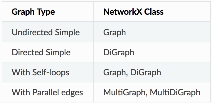
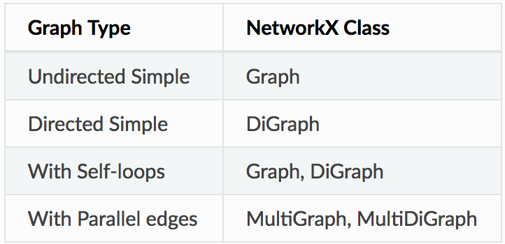
Certaines classes sont dédiées à des types de graphes spécifiques. Par exemple, la classe nx.DiGraph() permet de créer un graphe orienté.
Image('images/graphclasses.PNG', width = 400)
 Pour une liste complète des méthodes de création de graphes, réfère-toi à la documentation complète.
Accéder aux arêtes et aux nœuds
Tous les nœuds et toutes les arêtes d'un graphe sont accessibles à l'aide des méthodes G.nodes() et G.edges(). Les nœuds et arêtes individuels sont accessibles via la notation entre crochets (indexation).
G.nodes()
NodeView((1, 2, 3))
G.edges()
EdgeView([(1, 2), (1, 3), (2, 3)])
G[1] # same as G.adj[1]
AtlasView({2: {}, 3: {}})
G[1][2]
{}
G.edges[1, 2]
{}
👉 Visualisation de graphes avec Python
NetworkX fournit des fonctionnalités de base pour visualiser les graphes, mais son objectif principal est de permettre l'analyse de graphes plutôt que leur visualisation. Matplotlib propose des fonctions pratiques un peu plus avancées pour cela.
%matplotlib inline
import matplotlib.pyplot as plt
nx.draw(G)
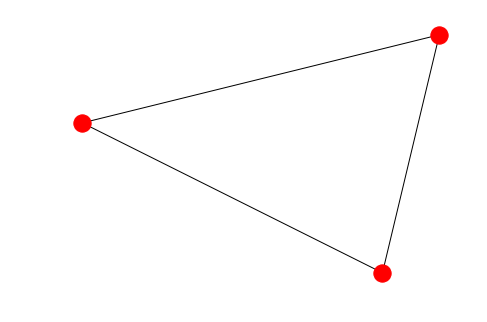 Ce bon vieux MatPlotLib peut nous mener loin pour visualiser des graphes. Cependant, des paquets dédiés comme
GraphViz sont probablement une meilleure option. GraphViz offre une interface Python via PyGraphViz, que tu dois installer pour l'utiliser (documentation complète).
import pygraphviz as pgv
d={'1': {'2': None}, '2': {'1': None, '3': None}, '3': {'1': None}}
A = pgv.AGraph(data=d)

print(A) # A is the simple representation of the graph as a string
strict graph "" {
	1 -- 2;
	2 -- 3;
	3 -- 1;
}
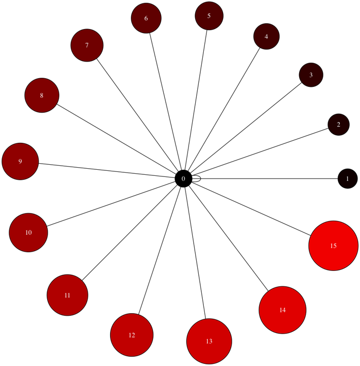
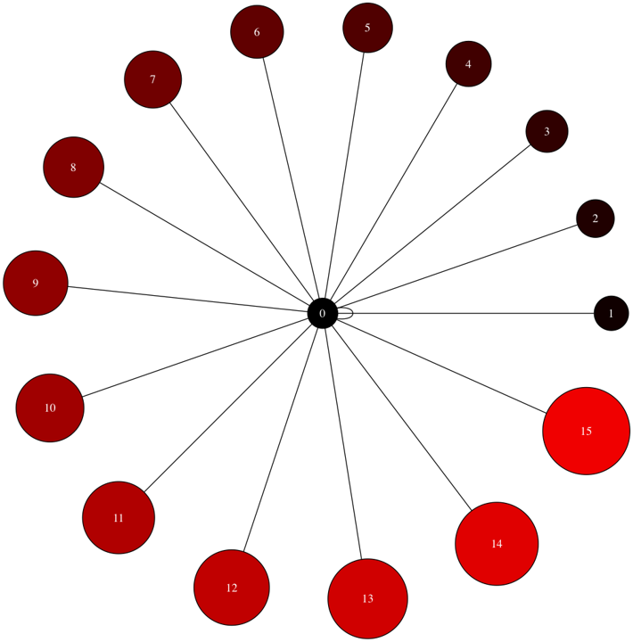
PyGraphviz offre un grand contrôle sur les attributs individuels des arêtes et des nœuds. On peut obtenir de très belles visualisations grâce à lui.
# Let's create another Graph where we can individually control the color of each node
B = pgv.AGraph()

# Setting node attributes that are common to all nodes
B.node_attr['style']='filled'
B.node_attr['shape']='circle'
B.node_attr['fixedsize']='true'
B.node_attr['fontcolor']='#FFFFFF'

# Creating and setting node attributes that vary for each node (using a for loop)
for i in range(16):
 B.add_edge(0,i)
 n=B.get_node(i)
 n.attr['fillcolor']="#%2x0000"%(i*16)
 n.attr['height']="%s"%(i/16.0+0.5)
 n.attr['width']="%s"%(i/16.0+0.5)
B.draw('star.png',prog="circo") # This creates a .png file in the local directory. Displayed below.

Image('images/star.png', width=650) # The Graph visualization we created above.
👉 Exploration d'un jeu de données avec des graphes
Pourquoi explorer avec des graphes ?
Considérons un jeu de données générique, c'est-à-dire un jeu de données qui n'a pas été spécifiquement construit pour l'analyse de graphes. Nous allons le transformer, à l'aide de pandas, en un jeu de données qui peut être géré sous forme de graphes. Notre cas d'étude est un jeu de données qui contient des itinéraires de compagnies aériennes. Pour chaque vol, il fournit l'aéroport de départ et l'aéroport d'arrivée ainsi que leurs horaires respectifs. On peut facilement imaginer ce jeu de données comme un graphe où les villes sont les arêtes et les connexions entre les villes (les routes) comme les arêtes. Cela peut aider à répondre à des questions comme :
- Quel est le chemin le plus court pour aller de l'aéroport A à l'aéroport B, que ce soit en distance ou en temps ?
- Existe-t-il un itinéraire pour aller de l'aéroport C à l'aéroport D ?
- Quels aéroports ont le trafic le plus chargé ?
- Quels aéroports sont les plus « centraux » par rapport aux autres ? Autrement dit, quels aéroports sont les plus connectés aux autres ?
Import du jeu de données et explorations de base
import pandas as pd
import numpy as np

data = pd.read_csv('https://raw.githubusercontent.com/mansont/datasets-tests/main/airlines.csv')
data.head()
 Quelques observations rapides sur le jeu de données étudié
L'information d'année, de mois, de jour et d'heure est répartie sur plusieurs colonnes. Nous voulons créer une seule colonne datetime contenant toutes les informations sur les horaires des vols. Nous devons aussi garder séparés l'heure prévue et l'heure réelle d'arrivée et de départ. Nous obtiendrons alors au final 4 colonnes datetime : heures prévue et réelle d'arrivée et de départ.
Tu peux aussi remarquer que les colonnes d'heure ne sont pas dans un format d'heure correct. Par exemple, 16:30 est représenté par 1630. Nous devrons régler cela à l'aide des expressions régulières.
Transformation des données
# converting sched_dep_time to 'std' - Scheduled time of departure
data['std'] = data.sched_dep_time.astype(str).str.replace('(\d{2}$)', '') + ':' + data.sched_dep_time.astype(str).str.extract('(\d{2}$)', expand=False) + ':00'

# converting sched_arr_time to 'sta' - Scheduled time of arrival
data['sta'] = data.sched_arr_time.astype(str).str.replace('(\d{2}$)', '') + ':' + data.sched_arr_time.astype(str).str.extract('(\d{2}$)', expand=False) + ':00'

# converting dep_time to 'atd' - Actual time of departure
data['atd'] = data.dep_time.fillna(0).astype(np.int64).astype(str).str.replace('(\d{2}$)', '') + ':' + data.dep_time.fillna(0).astype(np.int64).astype(str).str.extract('(\d{2}$)', expand=False) + ':00'

# converting arr_time to 'ata' - Actual time of arrival
data['ata'] = data.arr_time.fillna(0).astype(np.int64).astype(str).str.replace('(\d{2}$)', '') + ':' + data.arr_time.fillna(0).astype(np.int64).astype(str).str.extract('(\d{2}$)', expand=False) + ':00'
Maintenant que nous avons les colonnes d'heure au format voulu, nous pouvons vouloir combiner les colonnes year, month et day en une colonne de date. Ce n'est pas une étape absolument nécessaire, mais elle peut être pratique, et il restera toujours possible d'extraire l'information d'année, de mois et de jour quand nous le voudrons, une fois celle-ci convertie au format datetime.
data['date'] = pd.to_datetime(data[['year', 'month', 'day']])

# finally we drop the columns we don't need anymore
data = data.drop(columns = ['year', 'month', 'day'])
👉 Exploration avec NetworkX
Nous pouvons maintenant utiliser NetworkX pour importer directement le dataframe pandas sous forme de graphe. La fonction NetworkX pour ce faire est from_pandas_edgelist. La direction des vols est importante, nous devons donc indiquer à la fonction de considérer les arêtes comme ordonnées du départ vers l'arrivée.
Pour cela, nous utilisons les paramètres source et target. Les valeurs de la colonne indiquée dans « source » seront considérées comme les sommets d'origine, reliés par des arcs aux valeurs de la colonne indiquée dans « target ».
import networkx as nx
FG = nx.from_pandas_edgelist(data, source='origin', target='dest', edge_attr=True,)
Affichons les nœuds de notre nouveau graphe
FG.nodes()
NodeView(('EWR', 'MEM', 'LGA', 'FLL', 'SEA', 'JFK', 'DEN', 'ORD', 'MIA', 'PBI', 'MCO', 'CMH', 'MSP', 'IAD', 'CLT', 'TPA', 'DCA', 'SJU', 'ATL', 'BHM', 'SRQ', 'MSY', 'DTW', 'LAX', 'JAX', 'RDU', 'MDW', 'DFW', 'IAH', 'SFO', 'STL', 'CVG', 'IND', 'RSW', 'BOS', 'CLE'))
FG.edges()
EdgeView([('EWR', 'MEM'), ('EWR', 'SEA'), ('EWR', 'MIA'), ('EWR', 'ORD'), ('EWR', 'MSP'), ('EWR', 'TPA'), ('EWR', 'MSY'), ('EWR', 'DFW'), ('EWR', 'IAH'), ('EWR', 'SFO'), ('EWR', 'CVG'), ('EWR', 'IND'), ('EWR', 'RDU'), ('EWR', 'IAD'), ('EWR', 'RSW'), ('EWR', 'BOS'), ('EWR', 'PBI'), ('EWR', 'LAX'), ('EWR', 'MCO'), ('EWR', 'SJU'), ('LGA', 'FLL'), ('LGA', 'ORD'), ('LGA', 'PBI'), ('LGA', 'CMH'), ('LGA', 'IAD'), ('LGA', 'CLT'), ('LGA', 'MIA'), ('LGA', 'DCA'), ('LGA', 'BHM'), ('LGA', 'RDU'), ('LGA', 'ATL'), ('LGA', 'TPA'), ('LGA', 'MDW'), ('LGA', 'DEN'), ('LGA', 'MSP'), ('LGA', 'DTW'), ('LGA', 'STL'), ('LGA', 'MCO'), ('LGA', 'CVG'), ('LGA', 'IAH'), ('FLL', 'JFK'), ('SEA', 'JFK'), ('JFK', 'DEN'), ('JFK', 'MCO'), ('JFK', 'TPA'), ('JFK', 'SJU'), ('JFK', 'ATL'), ('JFK', 'SRQ'), ('JFK', 'DCA'), ('JFK', 'DTW'), ('JFK', 'LAX'), ('JFK', 'JAX'), ('JFK', 'CLT'), ('JFK', 'PBI'), ('JFK', 'CLE'), ('JFK', 'IAD'), ('JFK', 'BOS')])
Maintenant, visualisons le graphe avec draw_networkx.
# Quick view of the Graph
nx.draw_networkx(FG, with_labels=True)
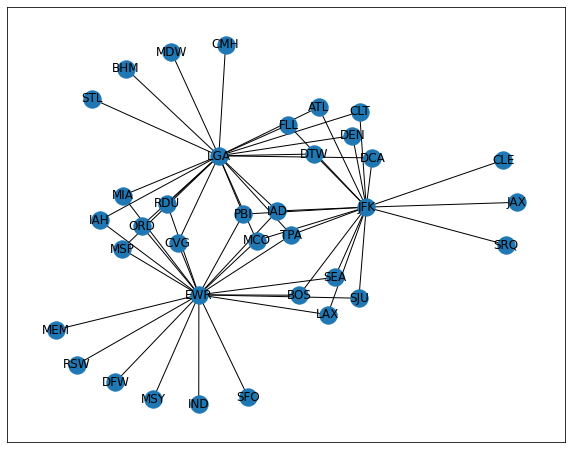 On peut facilement remarquer 3 aéroports qui sont centraux à toutes les routes enregistrées dans notre jeu de données.
👉 Identification des plus courts chemins
D'après le graphe ci-dessus, tu peux voir qu'il existe plusieurs chemins de certains aéroports vers d'autres. Il pourrait être intéressant d'identifier le plus court chemin entre 2 aéroports dans ce cas. On peut vouloir identifier à la fois le plus court chemin en distance et le plus court chemin en durée de vol.
Pour ce faire, nous devons d'abord pondérer les chemins avec l'une des deux métriques qui nous intéressent : la distance ou la durée. Pour notre illustration, considérons le temps comme la métrique que nous voulons analyser et utilisons-le comme poids (weight : valeur attribuée à une arête) pour les arêtes de notre graphe. Disons que nous voulons identifier le plus court chemin entre l'aéroport de Jacksonville, en Floride (JAX), et l'aéroport de Dallas/Fort Worth, au Texas (DFW).
Identifier tous les chemins disponibles
# Identify and display all paths available between these 2 points
for path in nx.all_simple_paths(FG, source='JAX', target='DFW'):
 print(path)
Algorithme de Dijkstra
L'algorithme de Dijkstra nous permet de trouver le plus court chemin entre deux sommets quelconques d'un graphe, qui sont souvent, dans les applications réelles, des réseaux routiers. NetworkX contient une implémentation de l'algorithme de Dijkstra que nous pouvons utiliser sans effort.
Description fondamentale du fonctionnement de l'algorithme de Dijkstra
# Dijkstra's path from JAX to DFW
dijk_path = nx.dijkstra_path(FG, source='JAX', target='DFW')
dijk_path
['JAX', 'JFK', 'SEA', 'EWR', 'DFW']
La route la plus courte de JAX à DFW en termes de distance comprend une escale aux aéroports de New York, dans l'État de New York (JFK), de Seattle, dans l'État de Washington (SEA), et de Newark, dans le New Jersey (EWR). Serait-ce la même chose si nous considérions la durée de vol (temps en vol) plutôt que la distance ?
# Let us try to find the dijkstra path weighted by airtime (approximate case)
shortpath = nx.dijkstra_path(FG, source='JAX', target='DFW', weight='air_time')
shortpath
['JAX', 'JFK', 'BOS', 'EWR', 'DFW']
La route la plus courte de JAX à DFW en termes de durée est légèrement différente de la route la plus courte en distance : au lieu d'une escale à Seattle, dans l'État de Washington (SEA), il nous faudrait faire un saut rapide de New York à Boston, dans le Massachusetts (BOS). Note que nous ne prenons pas en compte la durée des escales ici. Nous ne tenons compte que de la durée du vol, c'est-à-dire du temps en vol d'un aéroport à l'autre.
☝️ Résumé
Les graphes sont des structures mathématiques utilisées pour étudier les relations deux à deux entre des objets et des entités. Ils ont un large éventail d'applications dans divers défis du monde réel, comme l'étude des réseaux de compagnies aériennes, des réseaux sociaux, des transactions bancaires, etc. Nous pouvons explorer et visualiser un graphe avec Python à l'aide de paquets comme NetworkX, PyGraphViz et MatPlotLib. NetworkX est livré avec une multitude de fonctions pratiques qui nous permettent d'ingérer des dataframes sous forme de graphes, de les explorer et de les visualiser. Il nous permet aussi de réaliser des opérations avancées comme l'identification des plus courts chemins, ou l'algorithme de Dijkstra, d'un nœud à un autre en utilisant le poids de notre choix. Nous avons appliqué cela à l'exploration d'un jeu de données d'informations sur les compagnies aériennes et avons pu identifier le plus court chemin entre deux aéroports en termes de distance et en termes de durée de temps en vol.
💪 Challenge
Rends-toi sur le notebook Colab suivant. Fais une copie du notebook, réponds aux questions et partage le lien vers ton notebook dans cette quête.
📚 Plus de ressources
Introduction
“A picture speaks a thousand words” is one of the most commonly used phrases. But a graph speaks so much more than that. A visual representation of data, in the form of graphs, helps us gain actionable insights and make better data driven decisions based on them.
🤓 By the end of this quest, you will:
✅ Understand some common applications of graphs ✅ Know how to create and manage graphs with Python ✅ Understand how to use GraphViz to visualize graphs
👀 Content of the quest:
- Graph definition refresher
- Common applications of graphs
- Graphs creation with Python
- Graph visualization with Python
- Dataset exploration with graphs
- Exploring with NetworkX
- Identifying shortest paths
👉 Graph definition refresher
Basic definition of a graph
Graphs are mathematical structures used to study pairwise relationships between objects and entities. It is a branch of Discrete Mathematics and has found multiple applications in Computer Science, Chemistry, Linguistics, Operations Research, Sociology etc. I goes the same with Data Science and Analytics where graphs are used to model various structures and problems.
Let's look at a simple graph to review the concept. Look at the image below. Consider that this graph represents the places in a city that people generally visit, and the path that was followed by a visitor of that city.
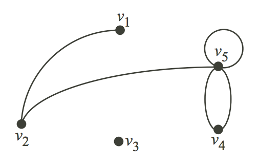
Let's consider V as the places and E as the path to travel from one place to another.
V = {v1, v2, v3, v4, v5}

E = {(v1,v2), (v2,v5), (v5, v5), (v4,v5), (v4,v4)}
Here, the edge (u,v) is the same as the edge (v,u) : they are unordered pairs.
Formally, a graph is a pair of sets such as G = (V,E). V is the set of vertices and E, a set of edges. E is made up of pairs of elements from V (unordered pair). In some cases, it is important to consider the edges as ordered pairs. Usually the edges are called arcs in such cases to indicate the notion of direction and these graphs are referred to as digraphs. Formally, a digraph is a pair of sets such as D = (V,A). V is the set of vertices and A, the set of arcs. A is made up of pairs of elements from V (ordered pair).
In a digraph, (u,v) is different from (v,u).
R and Python provide packages to analyze data using graph theory concepts. In this quest we will use the Python Package NetworkX.
Components of a graph
Python keeps at hand quick refreshers about graphs that we can access using the native package display. Here is for instance, a summary of the composition of graph. Note that Graph and Network are used interchangeably here. There is no difference between the two if not the necessity to consider network as the (programmatic) implementation of a (mathematical) graph.
from IPython.display import Image
Image('images/network.PNG')
👉 Common applications of graphs
Graphs are widely used to model, analyze and solve real-life problems. Here, you can find a few examples of noticeable applications of graph theories to some common problems.
Image('images/usecase.PNG')
A few more applications that are worth citing:
- Marketing Analytics: graphs can be used to figure out the most influential people in a social network. Advertisers and Marketers can so estimate the best performance for their marketing campaigns by routing their message through the most influential people.
- Banking Transactions: graphs can be used to find unusual patterns helping in mitigating fraudulent transactions. In some cases funding of terrorism activity has been detected by analyzing the flow of money across interconnected banking networks.
- Supply Chain: graphs help to identify optimal routes for delivery trucks and the optimal locations for warehouses and delivery centres
- Telecom: Telecom companies typically use graphs (Voronoi diagrams) to optimize coverage of cell towers on a given geographical surface
👉 Graphs creation with Python
We will use the networkx package in Python. This package needs to be installed before use.
Let's look at some common operations that we can do with the Networkx package.
Graph creation
import networkx as nx

# Create a Graph
G = nx.Graph() # This create a Graph object G but it is empty for now

# Add a node
G.add_node(1)

# Add a list of nodes by passing a list argument
G.add_nodes_from([2,3])

# Add edges between nodes
G.add_edge(1,2)

e = (2,3)
G.add_edge(*e) # the symbol * is used to unpack the tuple

# We can add edges using lists as well
G.add_edges_from([(1,2), (1,3)])
Here are some additional NetworkX function that can come in handy to create, process and manage graphs:
| Function | Description |
|---|---|
| subgraph(G, nbunch) | Display a subgraph view of G on nodes in nbunch |
| union(G1, G2) | Return a graph that is the union of graph G1 and G2 |
| disjoint_union(G1, G2) | Apply union on graphs G1 and G2 assuming all their nodes are different |
| cartesian_product(G1, G2) | Return the Cartesian product of 2 graphs G1 and G2 |
| compose(G1, G2) | Combine graphs identifying nodes common to both |
| complement(G) | Return the complement, that is, the inverse of the graph G |
| create_empty_copy(G) | Return an empty copy of a given graph |
| convert_to_undirected(G) | Return an undirected version of the graph G |
| convert_to_directed(G) | Return a directed representation of the graph G |
Some classes are dedicated to specific types of graphs. For example the nx.DiGraph() class allows to create a Directed Graph.
Image('images/graphclasses.PNG', width = 400)
 For a full list of Graph creation methods please refer to the full documentation.
Accessing edges and nodes
All nodes and edges of a graph can be accessed using the methods G.nodes() and G.edges(). Individual nodes and edges can be accessed using the bracket/subscript notation.
G.nodes()
NodeView((1, 2, 3))
G.edges()
EdgeView([(1, 2), (1, 3), (2, 3)])
G[1] # same as G.adj[1]
AtlasView({2: {}, 3: {}})
G[1][2]
{}
G.edges[1, 2]
{}
👉 Graph visualization with Python
NetworkX provides basic functionalities for visualizing graphs, but its main goal is to enable graph analysis rather than perform graph visualization. Matplotlib offers some more advanced convenient functions for this.
%matplotlib inline
import matplotlib.pyplot as plt
nx.draw(G)
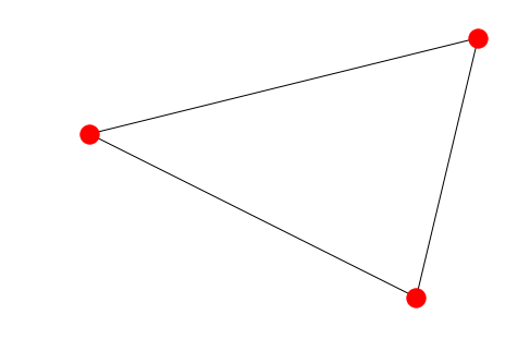 The old good MatPlotLib can go a long way helping us visualizing graphs. However, dedicated packages like
GraphViz are probably a better option. GraphViz offers a Python interface through PyGraphViz that you need to install to use (Full Documentation).
import pygraphviz as pgv
d={'1': {'2': None}, '2': {'1': None, '3': None}, '3': {'1': None}}
A = pgv.AGraph(data=d)

print(A) # A is the simple representation of the graph as a string
strict graph "" {
	1 -- 2;
	2 -- 3;
	3 -- 1;
}
PyGraphviz provides great control over the individual attributes of the edges and nodes. We can get very beautiful visualizations using it.
# Let's create another Graph where we can individually control the color of each node
B = pgv.AGraph()

# Setting node attributes that are common to all nodes
B.node_attr['style']='filled'
B.node_attr['shape']='circle'
B.node_attr['fixedsize']='true'
B.node_attr['fontcolor']='#FFFFFF'

# Creating and setting node attributes that vary for each node (using a for loop)
for i in range(16):
 B.add_edge(0,i)
 n=B.get_node(i)
 n.attr['fillcolor']="#%2x0000"%(i*16)
 n.attr['height']="%s"%(i/16.0+0.5)
 n.attr['width']="%s"%(i/16.0+0.5)
B.draw('star.png',prog="circo") # This creates a .png file in the local directory. Displayed below.

Image('images/star.png', width=650) # The Graph visualization we created above.
👉 Dataset exploration with graphs
Why exploring with graphs?
Let's consider a generic dataset, that is, a dataset that has not been specifically built for graph analysis. We will transform it, using pandas, into a dataset that can be manages as graphs. Our case study is a dataset that contains airlines routes. For each flight, it provides the airport of departure and the airport of arrival along with their respective times. We can easily imagine this dataset as a graph where the cities are the edges and connections between cities (the routes) as the edges. This can help address questions like:
- What is the shortest way to get from airport A to airport B, either in terms of distance or in terms of time?
- Is there a route to go from airport C to airport D?
- Which airports have the busiest traffic?
- Which airports are most "central" compared to the others? In other word, which airports are the most connected to the others?
Dataset import and basic explorations
import pandas as pd
import numpy as np

data = pd.read_csv('https://raw.githubusercontent.com/mansont/datasets-tests/main/airlines.csv')
data.head()
 A few quick observations about the dataset at hand
The year, month, day and time information is spread over several columns. We want to create one datetime column containing all information about the flights times. We also need to keep scheduled and actual time of arrival and departure separate. We will then end up with 4 datetime columns: scheduled and actual times of arrival and departure)
You can also notice that, the time columns are not in a proper time format. For instance, 16:30 is represented as 1630. We will need to address this using regular expressions.
Data transformation
# converting sched_dep_time to 'std' - Scheduled time of departure
data['std'] = data.sched_dep_time.astype(str).str.replace('(\d{2}$)', '') + ':' + data.sched_dep_time.astype(str).str.extract('(\d{2}$)', expand=False) + ':00'

# converting sched_arr_time to 'sta' - Scheduled time of arrival
data['sta'] = data.sched_arr_time.astype(str).str.replace('(\d{2}$)', '') + ':' + data.sched_arr_time.astype(str).str.extract('(\d{2}$)', expand=False) + ':00'

# converting dep_time to 'atd' - Actual time of departure
data['atd'] = data.dep_time.fillna(0).astype(np.int64).astype(str).str.replace('(\d{2}$)', '') + ':' + data.dep_time.fillna(0).astype(np.int64).astype(str).str.extract('(\d{2}$)', expand=False) + ':00'

# converting arr_time to 'ata' - Actual time of arrival
data['ata'] = data.arr_time.fillna(0).astype(np.int64).astype(str).str.replace('(\d{2}$)', '') + ':' + data.arr_time.fillna(0).astype(np.int64).astype(str).str.extract('(\d{2}$)', expand=False) + ':00'
Now that we have time columns in the format we wanted, we may want to combine the year, month and day columns into a date column. This is not an absolutely necessary step but it could be practical and it will still be possible to extract the year, month and day information when we want it once it's been converted into datetime format.
data['date'] = pd.to_datetime(data[['year', 'month', 'day']])

# finally we drop the columns we don't need anymore
data = data.drop(columns = ['year', 'month', 'day'])
👉 Exploring with NetworkX
We can now use networkx to import the pandas dataframe directly as a graph.The networkx function to do so is from_pandas_edgelist. The direction of the flights is important so we need to indicate to the function to consider the edges as ordered from departure to arrival.
For this, we use the parameters source and target. The values of the column indicated in "source" will be considered as the origin vertices connected with arcs to the values of the column indicated in "target".
import networkx as nx
FG = nx.from_pandas_edgelist(data, source='origin', target='dest', edge_attr=True,)
Display our new graph nodes
FG.nodes()
NodeView(('EWR', 'MEM', 'LGA', 'FLL', 'SEA', 'JFK', 'DEN', 'ORD', 'MIA', 'PBI', 'MCO', 'CMH', 'MSP', 'IAD', 'CLT', 'TPA', 'DCA', 'SJU', 'ATL', 'BHM', 'SRQ', 'MSY', 'DTW', 'LAX', 'JAX', 'RDU', 'MDW', 'DFW', 'IAH', 'SFO', 'STL', 'CVG', 'IND', 'RSW', 'BOS', 'CLE'))
FG.edges()
EdgeView([('EWR', 'MEM'), ('EWR', 'SEA'), ('EWR', 'MIA'), ('EWR', 'ORD'), ('EWR', 'MSP'), ('EWR', 'TPA'), ('EWR', 'MSY'), ('EWR', 'DFW'), ('EWR', 'IAH'), ('EWR', 'SFO'), ('EWR', 'CVG'), ('EWR', 'IND'), ('EWR', 'RDU'), ('EWR', 'IAD'), ('EWR', 'RSW'), ('EWR', 'BOS'), ('EWR', 'PBI'), ('EWR', 'LAX'), ('EWR', 'MCO'), ('EWR', 'SJU'), ('LGA', 'FLL'), ('LGA', 'ORD'), ('LGA', 'PBI'), ('LGA', 'CMH'), ('LGA', 'IAD'), ('LGA', 'CLT'), ('LGA', 'MIA'), ('LGA', 'DCA'), ('LGA', 'BHM'), ('LGA', 'RDU'), ('LGA', 'ATL'), ('LGA', 'TPA'), ('LGA', 'MDW'), ('LGA', 'DEN'), ('LGA', 'MSP'), ('LGA', 'DTW'), ('LGA', 'STL'), ('LGA', 'MCO'), ('LGA', 'CVG'), ('LGA', 'IAH'), ('FLL', 'JFK'), ('SEA', 'JFK'), ('JFK', 'DEN'), ('JFK', 'MCO'), ('JFK', 'TPA'), ('JFK', 'SJU'), ('JFK', 'ATL'), ('JFK', 'SRQ'), ('JFK', 'DCA'), ('JFK', 'DTW'), ('JFK', 'LAX'), ('JFK', 'JAX'), ('JFK', 'CLT'), ('JFK', 'PBI'), ('JFK', 'CLE'), ('JFK', 'IAD'), ('JFK', 'BOS')])
Now let's visualize the graph using draw_networkx.
# Quick view of the Graph
nx.draw_networkx(FG, with_labels=True)
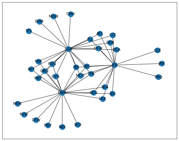 We can easily notice 3 airports that are central to all routes recorded in our dataset.
👉 Identifying shortest paths
From the graph above, you can see that there are multiple paths from some airports to others. It could be interesting to identify the shortest path between 2 airports that are in this case. We can want to identify both the shortest path in terms of distance and the shortest path in terms of flight duration.
To do so, we need first to weigh the paths with one of the two metrics of interest: distance or duration. For our illustration, let's consider time as the metric we want to analyze and use it as the weight for our graph edges. Say, we want to identify the shortest path between the airport of Jaksonville, Florida (JAX) and the airport of Dallas/Forth Worth, Texas (DFW).
Identify all available paths
# Identify and display all paths available between these 2 points
for path in nx.all_simple_paths(FG, source='JAX', target='DFW'):
 print(path)
Dijkstra's algorithm
Dijkstra's algorithm allows us to find the shortest path between any two vertices of a graph, which are often, in real-life applications, road networks. NetworkX holds an implementation of Dijkstra's algorithm for us to use seamlessly.
Fundamental description of the operation of Dijkstra's algorithm
# Dijkstra's path from JAX to DFW
dijk_path = nx.dijkstra_path(FG, source='JAX', target='DFW')
dijk_path
['JAX', 'JFK', 'SEA', 'EWR', 'DFW']
The shortest route from JAX to DFW in terms of distance includes a stop at New York, New York (JFK), Seattle, Washington (SEA) and Newark, New Jersey (EWR) airports. Would that be the same if we were considering flight duration (air time) instead of distance?
# Let us try to find the dijkstra path weighted by airtime (approximate case)
shortpath = nx.dijkstra_path(FG, source='JAX', target='DFW', weight='air_time')
shortpath
['JAX', 'JFK', 'BOS', 'EWR', 'DFW']
The shortest route from JAX to DFW in terms of duration is slightly different from the shortest distance route: instead of a stop at Seattle, Washington (SEA), we would have to take a quick jump from New York to Boston, Massachussetts (BOS). Note that we do not consider the duration of the layovers here. We only take into account the duration of the flight, that is, the air time from one airport to the other.
☝️ Summary
Graphs are mathematical structures used to study pairwise relationships between objects and entities. It has a wide range of applications in various real-world challenges such as the study of airlines networks, social networks, banking transactions, etc. We can explore and visualize graph with Python using packages like NetworkX, PyGraphViz and MatPlotLib. NetworkX comes with a wealth of practical functions that allow us to ingest dataframes as graphs, explore and visualize them. It also allows us to make advanced operations like the identification of the shortest paths, or Dijkstra's algorithm, from one node to another using the weight of our choice. We applied this to the exploration of an airlines information dataset and could identify the shortest path between two airports in terms of distance and in terms of air time duration.
💪 Challenge
Go to the following Colab Notebook. Make a copy of the notebook, answer the questions, and share the link to your notebook in this quest.